分箱与聚合
我们已经讨论了 数据、标记、编码 和 编码类型。Altair API 的下一个重要部分是其数据分箱和聚合的方法。
import altair as alt
from vega_datasets import data
cars = data.cars()

cars.head()
| 名称 (Name) | 每加仑英里数 (Miles_per_Gallon) | 气缸数 (Cylinders) | 排量 (Displacement) | 马力 (Horsepower) | 重量(磅)(Weight_in_lbs) | 加速度 (Acceleration) | 年份 (Year) | 产地 (Origin) | |
|---|---|---|---|---|---|---|---|---|---|
| 0 | 雪佛兰 Chevelle Malibu | 18.0 | 8 | 307.0 | 130.0 | 3504 | 12.0 | 1970-01-01 | 美国 (USA) |
| 1 | 别克 Skylark 320 | 15.0 | 8 | 350.0 | 165.0 | 3693 | 11.5 | 1970-01-01 | 美国 (USA) |
| 2 | 普利茅斯 Satellite | 18.0 | 8 | 318.0 | 150.0 | 3436 | 11.0 | 1970-01-01 | 美国 (USA) |
| 3 | AMC Rebel SST | 16.0 | 8 | 304.0 | 150.0 | 3433 | 12.0 | 1970-01-01 | 美国 (USA) |
| 4 | 福特 Torino | 17.0 | 8 | 302.0 | 140.0 | 3449 | 10.5 | 1970-01-01 | 美国 (USA) |
Pandas 中的 Group-By
数据探索中的一个关键操作是 group-by,这在《Python Data Science Handbook》的 第 4 章 中有详细讨论。简而言之,group-by 将数据根据某种条件进行分割,在这些组内应用一些聚合操作,然后将数据重新合并在一起。
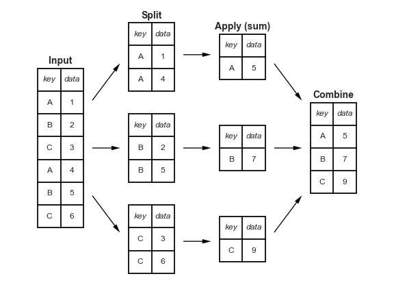
对于汽车数据,您可以按产地(Origin)进行分割,计算每加仑英里数(Miles per Gallon)的平均值,然后将结果合并。在 Pandas 中,该操作如下所示:
cars.groupby('Origin')['Miles_per_Gallon'].mean()
Origin
Europe    27.891429
Japan     30.450633
USA       20.083534
Name: Miles_per_Gallon, dtype: float64
在 Altair 中,这种分割-应用-合并的操作可以通过将聚合运算符作为字符串传递给任何编码来实现。例如,我们可以通过以下方式展示上述聚合操作的可视化:
alt.Chart(cars).mark_bar().encode(
    y='Origin',
    x='mean(Miles_per_Gallon)'
)
注意,分组操作隐式地在编码中完成:在这里,我们仅按产地(Origin)分组,然后计算每个组的平均值。
一维分箱:直方图
分箱最常见的用途之一是创建直方图。例如,这是每加仑英里数的直方图:
alt.Chart(cars).mark_bar().encode(
    alt.X('Miles_per_Gallon', bin=True),
    alt.Y('count()'),
    alt.Color('Origin')
)
Altair 声明式方法的一个有趣之处在于,它允许我们将这些值分配给不同的编码,以查看同一数据的其他视图。
例如,如果我们我们将分箱后的每加仑英里数映射到颜色上,我们将得到以下数据视图:
alt.Chart(cars).mark_bar().encode(
    color=alt.Color('Miles_per_Gallon', bin=True),
    x='count()',
    y='Origin'
)
这让我们更好地理解了每个国家内部每加仑英里数(MPG)的比例。
如果需要,我们可以将 x 轴上的计数进行归一化,以便直接比较比例。
alt.Chart(cars).mark_bar().encode(
    color=alt.Color('Miles_per_Gallon', bin=True),
    x=alt.X('count()', stack='normalize'),
    y='Origin'
)
我们可以看到,美国汽车中有超过一半属于“低油耗”类别。
再次改变编码,这次我们将颜色映射到计数上:
alt.Chart(cars).mark_rect().encode(
    x=alt.X('Miles_per_Gallon', bin=alt.Bin(maxbins=20)),
    color='count()',
    y='Origin',
)
现在我们看到了同一个数据集的热力图!
这正是 Altair 的一个美妙之处:它通过其 API 语法向您展示了不同图表类型之间的关系:例如,一个二维热力图与一个堆叠直方图编码的是相同的数据!
其他聚合
聚合也可以用于仅隐式分箱的数据。例如,请看这张随时间变化的每加仑英里数(MPG)图:
alt.Chart(cars).mark_point().encode(
    x='Year:T',
    color='Origin',
    y='Miles_per_Gallon'
)
点的重叠如此之多,使得很难看清数据的重要部分;我们可以通过绘制每个组的平均值(这里是每个年份/国家组合的平均值)使其更清晰。
alt.Chart(cars).mark_line().encode(
    x='Year:T',
    color='Origin',
    y='mean(Miles_per_Gallon)'
)
不过,mean 聚合只说明了一部分情况:Altair 还提供了内置工具来计算均值置信区间的下限和上限。
在这里,我们可以使用 mark_area(),并使用 y 和 y2 指定区域的下限和上限。
alt.Chart(cars).mark_area(opacity=0.3).encode(
    x='Year:T',
    color='Origin',
    y='ci0(Miles_per_Gallon)',
    y2='ci1(Miles_per_Gallon)'
)
时间分箱
一种特殊的分箱是将时间值按日期的某些方面进行分组:例如,一年中的月份或月中的天数。为了探索这一点,让我们看看一个包含西雅图平均气温的简单数据集:
temps = data.seattle_temps()
temps.head()
| 日期 (date) | 温度 (temp) | |
|---|---|---|
| 0 | 2010-01-01 00:00:00 | 39.4 |
| 1 | 2010-01-01 01:00:00 | 39.2 |
| 2 | 2010-01-01 02:00:00 | 39.0 |
| 3 | 2010-01-01 03:00:00 | 38.9 |
| 4 | 2010-01-01 04:00:00 | 38.8 |
如果我们尝试用 Altair 绘制这个数据,我们会得到一个 MaxRowsError。
alt.Chart(temps).mark_line().encode(
    x='date:T',
    y='temp:Q'
)
---------------------------------------------------------------------------
MaxRowsError                              Traceback (most recent call last)
/opt/hostedtoolcache/Python/3.7.7/x64/lib/python3.7/site-packages/altair/vegalite/v4/api.py in to_dict(self, *args, **kwargs)
    361         copy = self.copy(deep=False)
    362         original_data = getattr(copy, "data", Undefined)
--> 363         copy.data = _prepare_data(original_data, context)
    364
    365         if original_data is not Undefined:

/opt/hostedtoolcache/Python/3.7.7/x64/lib/python3.7/site-packages/altair/vegalite/v4/api.py in _prepare_data(data, context)
     82     # convert dataframes  or objects with __geo_interface__ to dict
     83     if isinstance(data, pd.DataFrame) or hasattr(data, "__geo_interface__"):
---> 84         data = _pipe(data, data_transformers.get())
     85
     86     # convert string input to a URLData

/opt/hostedtoolcache/Python/3.7.7/x64/lib/python3.7/site-packages/toolz/functoolz.py in pipe(data, *funcs)
    632     """
    633     for func in funcs:
--> 634         data = func(data)
    635     return data
    636

/opt/hostedtoolcache/Python/3.7.7/x64/lib/python3.7/site-packages/toolz/functoolz.py in __call__(self, *args, **kwargs)
    301     def __call__(self, *args, **kwargs):
    302         try:
--> 303             return self._partial(*args, **kwargs)
    304         except TypeError as exc:
    305             if self._should_curry(args, kwargs, exc):

/opt/hostedtoolcache/Python/3.7.7/x64/lib/python3.7/site-packages/altair/vegalite/data.py in default_data_transformer(data, max_rows)
     17 @curried.curry
     18 def default_data_transformer(data, max_rows=5000):
---> 19     return curried.pipe(data, limit_rows(max_rows=max_rows), to_values)
     20
     21

/opt/hostedtoolcache/Python/3.7.7/x64/lib/python3.7/site-packages/toolz/functoolz.py in pipe(data, *funcs)
    632     """
    633     for func in funcs:
--> 634         data = func(data)
    635     return data
    636

/opt/hostedtoolcache/Python/3.7.7/x64/lib/python3.7/site-packages/toolz/functoolz.py in __call__(self, *args, **kwargs)
    301     def __call__(self, *args, **kwargs):
    302         try:
--> 303             return self._partial(*args, **kwargs)
    304         except TypeError as exc:
    305             if self._should_curry(args, kwargs, exc):

/opt/hostedtoolcache/Python/3.7.7/x64/lib/python3.7/site-packages/altair/utils/data.py in limit_rows(data, max_rows)
     82             "than the maximum allowed ({}). "
     83             "For information on how to plot larger datasets "
---> 84             "in Altair, see the documentation".format(max_rows)
     85         )
     86     return data

MaxRowsError: The number of rows in your dataset is greater than the maximum allowed (5000). For information on how to plot larger datasets in Altair, see the documentation
alt.Chart(...)
len(temps)
8759
旁注:Altair 如何编码数据
我们选择对大于 5000 行的数据集引发 MaxRowsError,这是基于我们对学生使用 Altair 的观察,因为除非您考虑数据的表示方式,否则很容易导致笔记本变得非常庞大,从而影响性能。
当您将 Pandas 数据帧传递给 Altair 图表时,数据会被转换为 JSON 并存储在图表规范中。然后,这个规范会被嵌入到您笔记本的输出中,如果您用足够大的数据集以这种方式创建几十个图表,这会显著减慢您的机器速度。
那么如何绕过这个错误呢?有几种方法:
使用更小的数据集。例如,我们可以使用 Pandas 按天聚合温度数据。
import pandas as pd
temps = temps.groupby(pd.DatetimeIndex(temps.date).date).mean().reset_index()
使用以下方式禁用 MaxRowsError:
alt.data_transformers.enable('default', max_rows=None)
但请注意,如果不小心,这可能导致笔记本变得非常大。
从本地线程服务器提供数据。 altair data server 包使得这变得容易。
alt.data_transformers.enable('data_server')
请注意,此方法可能不适用于某些基于云的 Jupyter Notebook 服务。
使用指向数据源的 URL。创建一个
gist是存储常用数据的一种快速简便的方法。
我们在这里使用后一种方法,这是最方便且能带来最佳性能的。vega_datasets 中的所有数据源都包含一个 url 属性。
temps = data.seattle_temps.url
alt.Chart(temps).mark_line().to_dict()
{'config': {'view': {'continuousWidth': 400, 'continuousHeight': 300}},
 'data': {'url': 'https://vega.github.io/vega-datasets/data/seattle-temps.csv'},
 'mark': 'line',
 '$schema': 'https://vega.github.io/schema/vega-lite/v4.8.1.json'}
注意,这里只使用了 URL,而不是包含整个数据集。
现在我们再试试我们的图表:
alt.Chart(temps).mark_line().encode(
    x='date:T',
    y='temp:Q'
)
这个数据有点拥挤;假设我们想按月份对数据进行分箱。我们将使用 TimeUnit Transform 对日期进行此操作。
alt.Chart(temps).mark_point().encode(
    x=alt.X('month(date):T'),
    y='temp:Q'
)
如果我们现在对温度进行聚合,可能会更清晰:
alt.Chart(temps).mark_bar().encode(
    x=alt.X('month(date):O'),
    y='mean(temp):Q'
)
我们还可以通过两种不同的方式分割日期,以生成有趣的数据视图;例如:
alt.Chart(temps).mark_rect().encode(
    x=alt.X('date(date):O'),
    y=alt.Y('month(date):O'),
    color='mean(temp):Q'
)
或者我们可以查看按月份计算的小时平均温度:
alt.Chart(temps).mark_rect().encode(
    x=alt.X('hours(date):O'),
    y=alt.Y('month(date):O'),
    color='mean(temp):Q'
)
这种转换在处理时间数据时非常有用。
关于 TimeUnit Transform 的更多信息可在此处获得:https://vega-altair.cn/user_guide/transform/timeunit.html#user-guide-timeunit-transform